Label Format — OpenLABEL 1.0.0¶

Each scene variant ships a single label_OpenLABEL_style.json following the ASAM OpenLABEL 1.0.0 schema. It contains everything needed for cooperative perception: sensor declarations, the coordinate-system tree, per-frame agent poses, the raw sensor file URIs, and the 3D object annotations.

Top-level shape¶

{
  "openlabel": {
    "metadata":           { "schema_version": "1.0.0" },
    "streams":            { /* one entry per sensor — camera or lidar */ },
    "coordinate_systems": { /* scene → *_local → sensor_cs tree */ },
    "frames":             { "0": {...}, "1": {...}, ..., "100": {...} }
  }
}

flowchart TD
  frame["Frame f<br/>timestamp t"]
  frame --> streams["frame_properties.streams"]
  frame --> transforms["frame_properties.transforms"]
  frame --> objects["objects"]

  streams --> image_uri["camera URI<br/>images/agent/camera/image_f.png"]
  streams --> pcd_uri["lidar URI<br/>point_clouds/agent/lidar/.../point_cloud_f.pcd"]

  transforms --> scene_agent["scene → agent_local"]
  coord["coordinate_systems"] --> agent_sensor["agent_local → sensor_cs"]
  scene_agent --> chain["scene → sensor transform"]
  agent_sensor --> chain

  objects --> cuboid["cuboid<br/>x, y, z, qx, qy, qz, qw, L, W, H"]
  chain --> projection["projection / fusion"]
  image_uri --> projection
  pcd_uri --> projection
  cuboid --> projection

Streams¶

Each streams[<agent>/<sensor>] declares the sensor type and its intrinsics / resolution. See Sensors for a worked camera example.

Coordinate systems¶

A three-level tree links the scene frame to every sensor:

graph TD
  scene["scene (scene_cs)"]
  scene --> v10000["vehicle_10000_local (local_cs)"]
  scene --> v10010["vehicle_10010_local"]
  scene --> rsu1["rsu_1_local"]
  v10000 --> c9["vehicle_10000/camera_9_cs (sensor_cs)"]
  v10000 --> c10["vehicle_10000/camera_10_cs"]
  v10000 --> c11["vehicle_10000/camera_11_cs"]
  v10000 --> c12["vehicle_10000/camera_12_cs"]
  v10000 --> l5["vehicle_10000/lidar_5_cs"]

pose_wrt_parent on each sensor_cs is the sensor's extrinsic relative to its agent — constant over time (a calibration).
Per-frame agent poses live under frames[<id>].frame_properties.transforms as e.g. scene_to_vehicle_10000_local, each with { quaternion, translation }.
Vehicle-local and RSU-local frames are the parent frames for the sensors mounted on them.

flowchart LR
  scene["scene"]

  subgraph vehicle["vehicle_10000"]
    vlocal["vehicle_10000_local<br/>ego pose / parent frame"]
    vc9["camera_9_cs<br/>pose_wrt_parent"]
    vl5["lidar_5_cs<br/>pose_wrt_parent"]
    vlocal --> vc9
    vlocal --> vl5
  end

  subgraph rsu["rsu_1"]
    rlocal["rsu_1_local<br/>static pose / parent frame"]
    rc1["camera_1_cs<br/>pose_wrt_parent"]
    rl1["lidar_1_cs<br/>pose_wrt_parent"]
    rlocal --> rc1
    rlocal --> rl1
  end

  scene -- "frames[*].transforms<br/>scene_to_vehicle_10000_local" --> vlocal
  scene -- "coordinate_systems.rsu_1_local<br/>pose_wrt_parent" --> rlocal

Example sensor extrinsics:

"vehicle_10000/camera_9_cs": {
  "type": "sensor_cs",
  "parent": "vehicle_10000_local",
  "pose_wrt_parent": {
    "quaternion": [0.0, -0.0026, 0.0, 1.0],
    "translation": [-3.4916, 0.0, -1.6143]
  }
},
"vehicle_10000/lidar_5_cs": {
  "type": "sensor_cs",
  "parent": "vehicle_10000_local",
  "pose_wrt_parent": {
    "quaternion": [0.0, -0.0262, 0.0, 0.9997],
    "translation": [-1.0255, 0.0, -2.5021]
  }
}

The transform chain¶

To place a sensor (or its data) in the scene, compose the agent pose with the sensor's mounting extrinsic:

sensor_to_scene = local_to_scene(agent_local) ∘ sensor_to_local(sensor_cs)
scene_to_sensor = inverse(sensor_to_scene)

For vehicles, local_to_scene comes from the per-frame scene_to_vehicle_*_local transform (inverted).
For static RSUs, it usually comes from coordinate_systems[rsu_*_local].pose_wrt_parent.

The same chain applies to LiDAR: place the agent-local frame in the scene, then apply the LiDAR pose_wrt_parent.

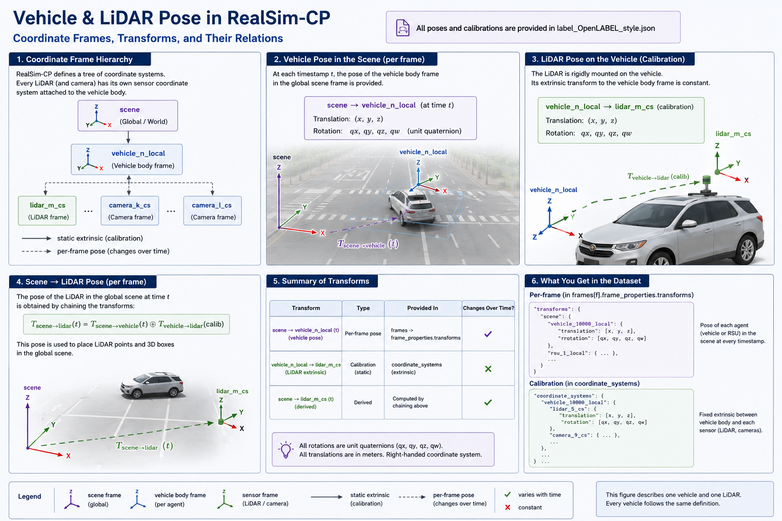
Vehicle and LiDAR pose transform chain

/// caption Expanded transform chain for one vehicle and one LiDAR. The vehicle pose changes per frame; the LiDAR mounting pose is a static calibration. Chaining both gives the LiDAR pose in the scene at that timestamp. ///

Frames¶

"frames": {
  "0": {
    "frame_properties": {
      "timestamp": 0.0,
      "streams":   { "vehicle_10000/camera_9": { "uri": "images/vehicle_10000/camera_9/image_000000.png" }, ... },
      "transforms":{ "scene_to_vehicle_10000_local": { "transform_src_to_dst": { "quaternion": [...], "translation": [...] } }, ... }
    },
    "objects": {
      "10040": {
        "object_data": {
          "type": "TYPE_PEDESTRIAN",
          "name": "TYPE_PEDESTRIAN_10040",
          "cuboid": {
            "name": "shape3D",
            "value": [ x, y, z,  qx, qy, qz, qw,  length, width, height ]
          }
        }
      }
    }
  }
}

Cuboid value vector (10 numbers)

[x, y, z, qx, qy, qz, qw, length, width, height] — position + orientation quaternion + extents, expressed in the scene frame. Note the xyzw quaternion order (not wxyz).

Vehicle pose origin vs. labeled cuboid¶

A connected vehicle's agent pose (vehicle_*_local) is the parent frame for its mounted sensors and sits near the rear-axle ground point — not the geometric body center. To draw the visible vehicle body, use its matching labeled object cuboid instead.

flowchart LR
  tf["frame_properties.transforms<br/>scene_to_vehicle_10000_local<br/>agent pose near rear tire bottom"]
  sensor["coordinate_systems<br/>vehicle_10000/*_cs<br/>camera/LiDAR mounting poses"]
  obj["objects['10000']<br/>cuboid.value<br/>center + quaternion + L/W/H"]
  viz["correct visualization<br/>vehicle body + sensors + projected data"]
  tf --> sensor
  tf --> viz
  sensor --> viz
  obj --> viz

For daiba_station_scenario/night_1, the vehicle_10000 cuboid is TYPE_MEDIUM_CAR, ~4.994 × 1.919 × 1.715 m. Expressed in vehicle_10000_local its center is about (1.379, 0.000, 0.857) — the z ≈ height/2 while x is well below length/2, confirming the agent pose is not the body center.

Object classes¶

The Daiba Station scenario uses: TYPE_PEDESTRIAN, TYPE_SMALL_CAR, TYPE_COMPACT_CAR, TYPE_MEDIUM_CAR, TYPE_LUXURY_CAR, TYPE_BUS. The full dataset spans 12 classes; see Benchmark for the complete list and the evaluation class mapping.